จาก ep ที่แล้วที่เราได้เรียนรู้ ว่า TensorFlow.js คืออะไร ใน ep นี้เราจะใช้ TensorFlow.js ในการสร้างโมเดล Neural Network ในงาน Classifier สำหรับข้อมูลแบบตาราง Tabular Data เราจะเทรนกับชุดข้อมูลดอกไอริส Iris Dataset ซึ่งถือว่าเป็นชุดข้อมูลที่ง่าย สำหรับ Machine Learning, Pattern Recognition
Tabular Data
ข้อมูลเพิ่มเติม งานประมวลผลข้อมูลแบบมีโครงสร้าง Structure Data ในรูปแบบ ตาราง Tabular Data ep.1
Iris Dataset
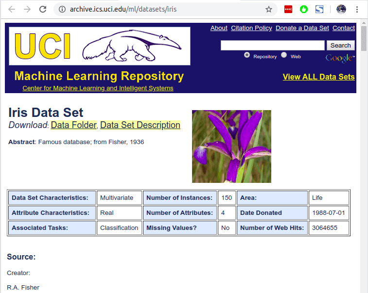
Iris Dataset คือ ชุดข้อมูลสำหรับงาน Pattern Recognition ที่แพร่หลายที่สุด เป็นงานคลาสสิกที่ยังถูกอ้างถึงจนถึงปัจจุบัน ใน Dataset ประกอบด้วย ข้อมูล ดอกไอริส 3 สายพันธุ์ สายพันธุ์ละ 50 ตัวอย่าง
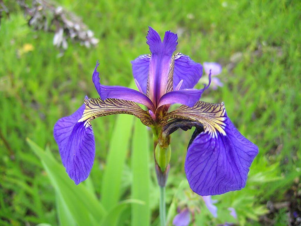

Iris Setosa 1. Credit https://commons.wikimedia.org/wiki/File:Irissetosa1.jpg 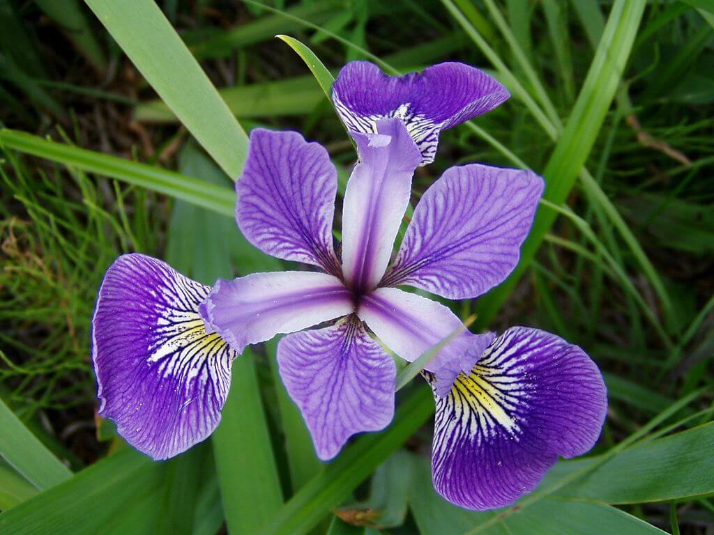
Blue flag flower close-up (Iris versicolor). Credit https://commons.wikimedia.org/wiki/File:Iris_versicolor_3.jpg 

image of Iris virginica shrevei BLUE FLAG at the James Woodworth Prairie Preserve – a bud and a single flower at full bloom. Credit https://commons.wikimedia.org/wiki/File:Iris_virginica.jpg
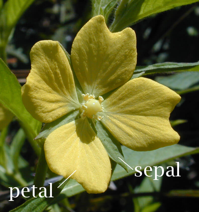
ให้เราทำนายสายพันธุ์จากข้อมูลกายภาพของกลีบดอก และกลีบเลี้ยง
คำอธิบาย Column ใน Dataset
- sepal length in cm ความยาวกลีบเลี้ยง (เซนติเมตร)
- sepal width in cm ความกว้างกลีบเลี้ยง (เซนติเมตร)
- petal length in cm ความยาวกลีบดอก (เซนติเมตร)
- petal width in cm ความกว้างกลีบดอก (เซนติเมตร)
- class: สายพันธุ์
- Iris Setosa
- Iris Versicolour
- Iris Virginica
ตัวอย่างข้อมูลใน Iris Dataset
sepal_length,sepal_width,petal_length,petal_width,species
5.1,3.5,1.4,0.2,setosa
4.9,3,1.4,0.2,setosa
4.7,3.2,1.3,0.2,setosa
4.6,3.1,1.5,0.2,setosa
5.4,3.9,1.7,0.4,setosa
7,3.2,4.7,1.4,versicolor
6.4,3.2,4.5,1.5,versicolor
6.9,3.1,4.9,1.5,versicolor
5.5,2.3,4,1.3,versicolor
6.5,2.8,4.6,1.5,versicolor
7.3,2.9,6.3,1.8,virginica
6.7,2.5,5.8,1.8,virginica
7.2,3.6,6.1,2.5,virginica
6.5,3.2,5.1,2,virginica
6.4,2.7,5.3,1.9,virginica
Iris Dataset Statistics:
Min Max Mean SD Class Correlation
sepal length: 4.3 7.9 5.84 0.83 0.7826
sepal width: 2.0 4.4 3.05 0.43 -0.4194
petal length: 1.0 6.9 3.76 1.76 0.9490 (high!)
TensorFlow.js Code Example
เริ่มต้นด้วยใส่ Code ด้านล่าง ไว้ระหว่าง HTML tag head และ body
<script src="https://cdn.jsdelivr.net/npm/@tensorflow/tfjs@latest"></script>ประกาศฟังก์ชัน run() ที่จะบรรจุ code ในการทำ Data Pipeline และเทรนโมเดล และ เรียกฟังก์ชัน run เมื่อเปิดหน้าเว็บ
    <script lang="js">
        async function run() {
            .
            .
            .
        }
        run();
    </script>
สร้าง Data Pipeline กำหนด Data Source ของข้อมูล ในที่นี้คือ ไฟล์ iris.csv ใช้ข้อมูลทั้งหมดเป็น Training Set และกำหนดให้ column species เป็น Label
เพื่อความง่าย ในเคสนี้ เราจะไม่ทำ Feature Engineering หรือ Normalization ใด ๆ เลย
ในส่วนของ Label เราจะแปลงค่าจาก String เช่น “setosa” ใน Dataset โดย Encode ด้วย One-Hot Encoding ให้เป็น array ขนาด 3 Element ตามจำนวน Class
แล้วสร้าง Data Loader ด้วย Batch Size ขนาด 16
            const csvUrl = 'data/iris.csv';
            const trainingData = tf.data.csv(csvUrl, {
                columnConfigs: {
                    species: {
                        isLabel: true
                    }
                }
            });

            const numOfFeatures = (await trainingData.columnNames()).length -1;
            const numOfSamples = 150;
            const convertedData = trainingData.map(({xs, ys}) => {
                const labels = [
                    ys.species == 'setosa' ? 1 : 0,
                    ys.species == 'virginica' ? 1 : 0,
                    ys.species == 'versicolor' ? 1 : 0,
                ]
                return { xs: Object.values(xs), ys: Object.values(labels)};
            }).batch(16);
สร้างโมเดล Neural Network แบบ Sequential ความลึก 2 Dense Layer Layer แรก มีขนาด 4 Neuron ใช้ ReLU Activation Function และ Layer Output ขนาด 3 Neuron ตามจำนวน Class โดยใช้ SoftMax Function
โมเดลนี้เป็นโมเดล แบบ Multi-Class Classification มี Output 3 Class (มากกว่า 2 หรือ Binary) เราจึงต้องใช้ Categorical Cross Entropy Loss Function และเราจะใช้ Adam Optimizer ด้วย Learning Rate 0.06
const model = tf.sequential();
model.add(tf.layers.dense({inputShape: [numOfFeatures], activation: 'relu', units: 4}))
model.add(tf.layers.dense({activation: 'softmax', units: 3}))
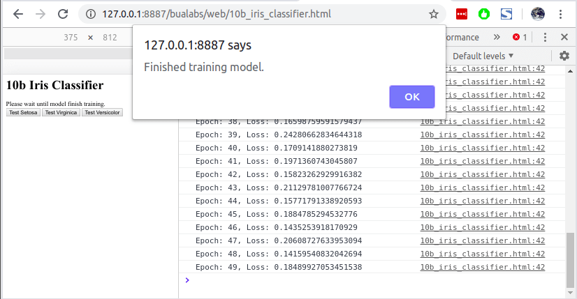
model.compile({loss: 'categoricalCrossentropy', optimizer: tf.train.adam(0.06)});สั่งให้เทรนไป 50 Epoch โดยทุก Epoch ให้ Callback กลับมา เพื่อ log ค่า Loss ใน Console เมื่อเทรนเสร็จเรียบร้อยให้ Alert บอก
            await model.fitDataset(convertedData,
                    {epochs: 50,
                     callbacks: {
                         onEpochEnd: async(epoch, logs) => {
                             console.log("Epoch: " + epoch + ", Loss: " + logs.loss);
                         }
                    }});
            alert("Finished training model.")
กำหนดฟังก์ชันสำหรับเทส การ Predict โดยนำข้อมูลตัวอย่าง 3 ตัวอย่างมาจากใน Training Set (ยังไม่สนใจเรื่อง Overfit)
        function testPredict(idx) {
            xs = [[4.3, 3,   1.1, 0.1],
                  [6.5, 3,   5.8, 2.2],
                  [6.6, 2.9, 4.6, 1.3],];
            testVal = tf.tensor2d(xs[idx], [1, 4]);

            const prediction = model.predict(testVal);
            const pIndex = tf.argMax(prediction, axis=1).dataSync();
            classNames = ["Setosa", "Virginica", "Versicolor"]

            alert(classNames[pIndex] + prediction)
        }
สร้างปุ่มสำหรับเรียกฟังก์ชัน testPredict() ด้านบน ตาม Index ที่กำหนด
        <button id="b0" name="b0" onclick="testPredict(0)">Test Setosa</button>
        <button id="b1" name="b1" onclick="testPredict(1)">Test Virginica</button>
        <button id="b2" name="b2" onclick="testPredict(2)">Test Versicolor</button>
เรามาเริ่มกันเลยดีกว่า
Training
เริ่มต้นเทรน เมื่อเปิดหน้าเว็บ ให้เรากด F12 เปิด Console ของ Web Browser ขึ้นมาจะเห็น ดังนี้
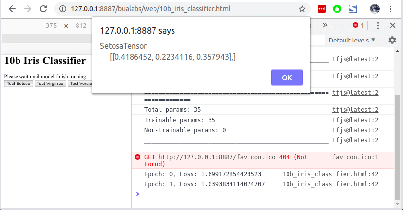
- Model Architecture สังเกตว่า มี 2 Dense Layer
- 4 Neuron มี 20 Param มาจาก 4 (Input Shape) x 4 (Weight) + 4 Bias
- 3 Neuron มี 15 Param มาจาก 4 (Input Shape) x 3 (Weight) + 3 (Bias)
- log จะมี เลขที่ Epoch 0-49 และ ค่า Loss ที่ลดลงเรื่อย ๆ
_________________________________________________________________
Layer (type)                 Output shape              Param #
=================================================================
dense_Dense1 (Dense)         [null,4]                  20
_________________________________________________________________
dense_Dense2 (Dense)         [null,3]                  15
=================================================================
Total params: 35
Trainable params: 35
Non-trainable params: 0
_________________________________________________________________

Epoch: 0, Loss: 1.5627639293670654
Epoch: 1, Loss: 0.9489914178848267
Epoch: 2, Loss: 0.9920297265052795
Epoch: 3, Loss: 0.7840166687965393
Epoch: 4, Loss: 0.6871854066848755
Epoch: 5, Loss: 0.61978679895401
Epoch: 6, Loss: 0.5794975757598877
Epoch: 7, Loss: 0.5294687747955322
Epoch: 8, Loss: 0.530101478099823
Epoch: 9, Loss: 0.5019513964653015
Epoch: 10, Loss: 0.429468035697937
....
Epoch: 46, Loss: 0.1435253918170929
Epoch: 47, Loss: 0.20608727633953094
Epoch: 48, Loss: 0.14159540832042694
Epoch: 49, Loss: 0.18489927053451538
Alert เมื่อโมเดลเทรน ครบจำนวน Epoch ที่กำหนด
Inference
เราสามารถกดปุ่มให้โมเดล Predict ได้เลย โดยไม่ต้องรอให้โมเดลเทรนเสร็จ แต่ค่าที่ Predict ได้จะไม่ต่างกับ Random
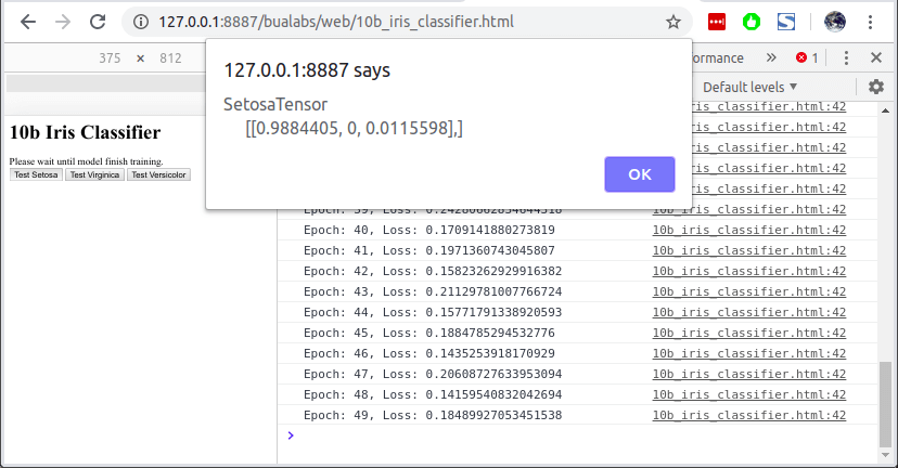
เมื่อเทรนเสร็จแล้ว เราสามารถกดปุ่ม Test Setosa เพื่อให้โมเดล Predict จากข้อมูล Setosa ที่เรากำหนดไว้ใน Function testPredict() โมเดลทำนายว่าเป็น Setosa ด้วยความน่าจะเป็น 98.84%
Network Request
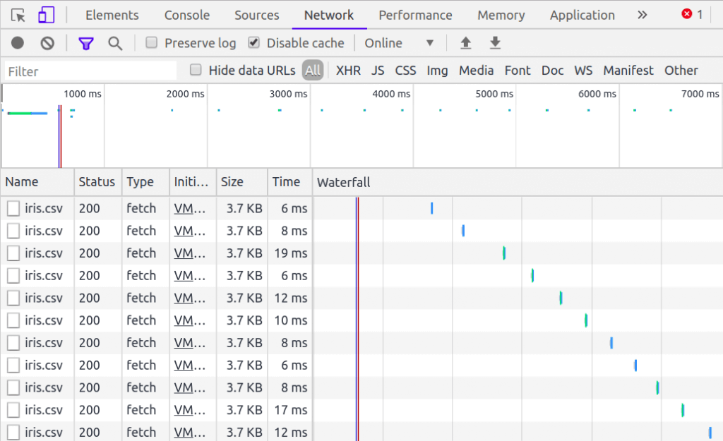
ปัญหาอย่างหนึ่งของ Data Pipeline ด้านบน คือ Web Browser จะยิง HTTP Request เพื่อ Download ไฟล์ iris.csv ใหม่ทุก Epoch ซึ่งเราจะแก้ปัญหานี้กันใน ep ต่อไป
Credit
- https://www.coursera.org/learn/browser-based-models-tensorflow
- https://archive.ics.uci.edu/ml/datasets/iris