จาก ep ที่แล้ว Multi-Class Classification สำหรับ Tabular Data ใน ep นี้เราจะใช้ TensorFlow.js ในการสร้างโมเดล Neural Network ในงาน Binary Classifier วินิจฉัยโรคมะเร็งเต้านม Breast Cancer Diagnostic จากชุดข้อมูล Breast Cancer Wisconsin (Diagnostic) Dataset จาก ซึ่งเป็นข้อมูลแบบตาราง Tabular Data จาก UCI : Center for Machine Learning and Intelligent Systems
Tabular Data
ข้อมูลเพิ่มเติม งานประมวลผลข้อมูลแบบมีโครงสร้าง Structure Data ในรูปแบบ ตาราง Tabular Data ep.1
Breast Cancer Wisconsin (Diagnostic) Dataset
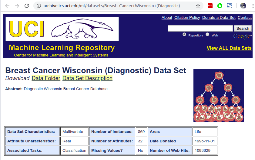
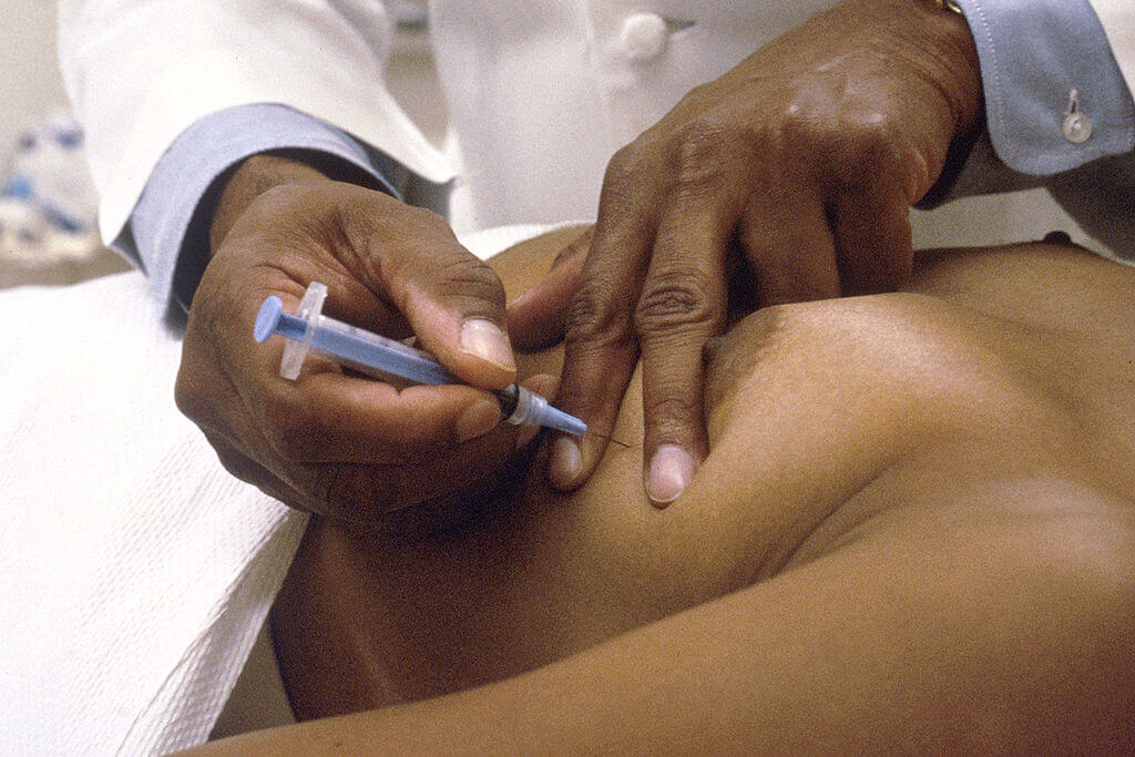
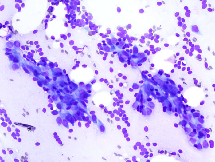
Breast Cancer Wisconsin (Diagnostic) Dataset คือ ชุดข้อมูลที่ประกอบด้วย Feature ต่าง ๆ ที่คำนวนมาจาก รูปดิจิตอลของ Fine Needle Aspiration (FNA) ของเซลล์เต้านม
Feature ต่าง ๆ จะบ่อบอกถึงคุณลักษณะของ Cell Nuclei ที่อยู่ในรูปภาพ ดังรูปตัวอย่างด้านล่าง
ให้เราวินิจฉัยโรคมะเร็งเต้านม Breast Cancer Diagnostic ใน Column ชื่อ diagnosis: B = Benign (เนื้องอกธรรมดา), M = Malignant (เนื้อร้าย) จากข้อมูล Input 30 Feature
Class distribution เท่ากับ 357 benign, 212 malignant จากทั้งหมด 569 ตัวอย่าง
คำอธิบาย Column ใน Dataset
- ID Number
- Diagnosis (M = malignant, B = benign)
และ Column ที่ 3 – 32 ประกอบด้วย
- radius (mean of distances from center to points on the perimeter)
- texture (standard deviation of gray-scale values)
- perimeter
- area
- smoothness (local variation in radius lengths)
- compactness (perimeter^2 / area – 1.0)
- concavity (severity of concave portions of the contour)
- concave points (number of concave portions of the contour)
- symmetry
- fractal dimension (“coastline approximation” – 1)
แต่ละรูป จะถูกคำนวนค่า Mean, Standard Error และ Worst หรือ Largest (Mean ของ 3 ค่า Largest) ของทั้ง 10 ข้อด้านบน ตัวอย่างเช่น Field 3 คือ Mean Radius, Field 13 คือ Radious Standard Error และ Field คือ Worst Radius
ในทุก Row ทุก Column ข้อมูลครบทุกช่อง ไม่มีข้อมูลขาดหาย และทุก Feature จะถูกบันทึกด้วยทศนิยม 4 ตำแหน่ง
ตัวอย่างข้อมูลใน WDBC Dataset
diagnosis,meanradius,meantexture,meanperimeter,meanarea,meansmoothness,meancompactness,meanconcavity,meanconcavepoints,meansymmetry,meanfractaldimension,seradius,setexture,seperimeter,searea,sesmoothness,secompactness,seconcavity,seconcavepoints,sesymmetry,sefractaldimension,worstradius,worsttexture,worstperimeter,worstarea,worstsmoothness,worstcompactness,worstconcavity,worstconcavepoints,worstsymmetry,worstfractaldimension
0,-1.150364822,-0.390641961,-1.128550208,-0.9587635786,0.3109837048,-0.5959945009,-0.8025961223,-0.8024900198,0.2945390619,0.09425149978,-0.4950522998,1.487201532,-0.5144878222,-0.4915400491,0.2814983704,-0.6045120643,-0.4690070058,-0.6117000235,0.05798237404,-0.3576370159,-1.043175598,0.2135328249,-1.036044595,-0.8488077145,0.3424985112,-0.7300974341,-0.8123205317,-0.757983665,-0.01614760641,-0.3850340195
0,-0.9379897202,0.6805140506,-0.9482014635,-0.8215254807,-0.6096360366,-0.9098672137,-0.6606690499,-0.8987161166,0.7549345255,-0.4254708237,-0.3338175654,0.7594120303,-0.2875180469,-0.4212769481,-0.1620796961,-0.2048669322,-0.05029632323,-0.2030907624,-0.2546900516,-0.3913946268,-0.715654153,1.066841832,-0.6899220458,-0.6686970251,-0.09553744619,-0.537866468,-0.3750480642,-0.6068702269,0.09669003693,-0.386157972
0,0.5741210021,-1.033335568,0.5139409811,0.408586269,-0.1061607801,-0.3630188613,-0.4179904837,-0.08844569488,-0.271820437,-0.5752213237,-0.5767257898,-1.057845105,-0.5385603741,-0.3870892303,-1.072118825,-0.7205749568,-0.423627908,-0.4921898782,-0.6748436235,-0.8014728771,0.2976153181,-0.977817827,0.262136649,0.1138881885,-0.5247241923,-0.5208664506,-0.1829891708,-0.02371948445,-0.200502066,-0.75144254
0,-0.5472195336,-0.316022104,-0.5776218521,-0.5666147977,0.5866617991,-0.6493310516,-0.8052982696,-0.5000651441,0.3310783844,0.5405667155,-0.128225677,0.556222068,-0.20400103,-0.3323469337,-0.55285085,-0.7588814287,-0.6489142092,0.6015656139,0.2045475736,-0.1159632107,-0.7013250898,-0.7579266598,-0.73573673,-0.6589659262,-0.8167481639,-1.034920823,-1.091633335,-0.8525445081,-1.076185749,-0.5468831819
0,-0.5273978574,0.79124029,-0.5615634023,-0.5235706692,-1.051446456,-1.017531701,-0.9051490476,-0.9358059599,-0.9697214968,-0.4269389659,-0.6288278437,-0.1309294409,-0.6132344127,-0.4665809177,-0.6714903805,-0.7440162306,-0.7100633481,-1.204497506,-0.542934944,-0.5030249082,-0.4270258794,1.058636937,-0.422423406,-0.4409551676,-0.3034939108,-0.4672510111,-0.7245651627,-0.7831181517,0.3112404855,-0.08212881608
TensorFlow.js Code Example
เริ่มต้นด้วยใส่ Code ด้านล่าง ไว้ระหว่าง HTML tag head และ body
<script src="https://cdn.jsdelivr.net/npm/@tensorflow/tfjs@latest"></script>ประกาศฟังก์ชัน run() ที่จะบรรจุ code ในการทำ Data Pipeline และเทรนโมเดล และ เรียกฟังก์ชัน run เมื่อเปิดหน้าเว็บ
    <script lang="js">
        async function run() {
            .
            .
            .
        }
        run();
    </script>
สร้าง Data Pipeline กำหนด Data Source ของข้อมูล ในที่นี้คือ ไฟล์ wdbc-train.csv ใน Folder data เป็น Training Set และไฟล์ wdbc-test.csv เป็น Validation Set โดยกำหนดให้ column diagnosis เป็น Label
เพื่อความง่าย ในเคสนี้ เราจะไม่ทำ Feature Engineering หรือ Normalization ใด ๆ เลย
ในส่วนของ Label เนื่องจากในเคสนี้เป็น Binary Classification แค่ 0 / 1 เราจึงไม่ต้องแปลงเป็น One-Hot Encoding
แล้วสร้าง Data Loader ด้วย Batch Size ขนาด 16
            const trainingUrl = 'data/wdbc-train.csv';

            const trainingData = tf.data.csv(trainingUrl, {
                columnConfigs: {
                    diagnosis: {
                        isLabel: true
                    }
                }
            });

            const convertedTrainingData = trainingData.map(({xs, ys}) => {
                return { xs: Object.values(xs), ys: Object.values(ys)};
            }).batch(16);

            const testingUrl = 'data/wdbc-test.csv';

            const testingData = tf.data.csv(testingUrl, {
                columnConfigs: {
                    diagnosis: {
                        isLabel: true
                    }
                }
            });

            const convertedTestingData = testingData.map(({xs, ys}) => {
                return { xs: Object.values(xs), ys: Object.values(ys)};
            }).batch(16);

            const numOfFeatures = (await trainingData.columnNames()).length - 1;
สร้างโมเดล Neural Network แบบ Sequential ความลึก 2 Dense Layer Layer แรก มีขนาด 8 Neuron ใช้ ReLU Activation Function และ Layer Output ขนาด 1 Neuron โดยใช้ Sigmoid Function เนื่องจากเป็นงาน Binary Classification
โมเดลนี้เป็นโมเดล แบบ Binary Classification มี Output 2 Class คือ 0 หรือ 1 เท่านั้น เราจึงต้องใช้ Binary Cross Entropy Loss Function และเราจะใช้ RMSProp Optimizer ด้วย Learning Rate 0.03
Metrics สำหรับวัดประสิทธิภาพของโมเดล กับข้อมูลใน Validation Set คือ Accuracy
            const model = tf.sequential();
            model.add(tf.layers.dense({inputShape: [numOfFeatures], activation: "relu", units: 8}))
            model.add(tf.layers.dense({activation: "sigmoid", units: 1}));

            model.compile({loss: "binaryCrossentropy", optimizer: tf.train.rmsprop(0.03), metrics: "accuracy"});
            model.summary()
สั่งให้เทรนไป 30 Epoch โดยทุก Epoch ให้ Callback กลับมา เพื่อ log ค่า Loss และ Accuracy ใน Console เมื่อเทรนเสร็จเรียบร้อยให้ Save โมเดลเก็บไว้
            await model.fitDataset(convertedTrainingData,
                             {epochs:30,
                              validationData: convertedTestingData,
                              callbacks:{
                                  onEpochEnd: async(epoch, logs) =>{
                                      console.log("Epoch: " + epoch + " Loss: " + logs.loss + " Accuracy: " + logs.acc);
                                  }
                              }});
            await model.save('downloads://my_model');
เรามาเริ่มกันเลยดีกว่า
Training
เริ่มต้นเทรน เมื่อเปิดหน้าเว็บ ให้เรากด F12 เปิด Console ของ Web Browser ขึ้นมาจะเห็น ดังนี้
- Model Architecture สังเกตว่า มี 2 Dense Layer
- 8 Neuron มี 248 Param มาจาก 30 (Input Shape) x 8 (Weight) + 8 Bias
- 1 Neuron มี 9 Param มาจาก 8 (Input Shape) x 1 (Weight) + 1 (Bias)
- log จะมี เลขที่ Epoch 0-29, ค่า Loss ที่ลดลงเรื่อย ๆ และ Accuracy ที่เพิ่มขึ้นเรื่อย ๆ จนถึงมากกว่า 99%
_________________________________________________________________
Layer (type)                 Output shape              Param #
=================================================================
dense_Dense1 (Dense)         [null,8]                  248
_________________________________________________________________
dense_Dense2 (Dense)         [null,1]                  9
=================================================================
Total params: 257
Trainable params: 257
Non-trainable params: 0
_________________________________________________________________

Epoch: 0 Loss: 0.1549004465341568 Accuracy: 0.9428570866584778
Epoch: 1 Loss: 0.06617123633623123 Accuracy: 0.9802197217941284
Epoch: 2 Loss: 0.05083293840289116 Accuracy: 0.9846153259277344
Epoch: 3 Loss: 0.04226241633296013 Accuracy: 0.9846153259277344
Epoch: 4 Loss: 0.03636830300092697 Accuracy: 0.9868131279945374
Epoch: 5 Loss: 0.03918159008026123 Accuracy: 0.9868131279945374
Epoch: 6 Loss: 0.031536202877759933 Accuracy: 0.9934065341949463
Epoch: 7 Loss: 0.027139972895383835 Accuracy: 0.9934065341949463
Epoch: 8 Loss: 0.025623716413974762 Accuracy: 0.9934065341949463
Epoch: 9 Loss: 0.022028112784028053 Accuracy: 0.9934065341949463
Epoch: 10 Loss: 0.01898837834596634 Accuracy: 0.9978021383285522
...
Epoch: 26 Loss: 0.005634100176393986 Accuracy: 0.9978021383285522
Epoch: 27 Loss: 0.003376677865162492 Accuracy: 0.9978021383285522
Epoch: 28 Loss: 0.004708329681307077 Accuracy: 0.9978021383285522
Epoch: 29 Loss: 0.0036777183413505554 Accuracy: 0.9978021383285522
Result
Accuracy: 99.78%
Credit
- https://www.coursera.org/learn/browser-based-models-tensorflow
- https://archive.ics.uci.edu/ml/datasets/Breast+Cancer+Wisconsin+(Diagnostic)